Construction of an eCE model

In order to construct an eCE model, one needs to specify the lattice and the degrees of freedom in addition to the chemical embedding and the energy model. The energy model is by default a feed forward fully connected neural network (FNN).

The commande build in the ece is meant for constructing an eCE model. Arguments can directly be given via the command line interface or via a YAML settings file. When both arguments are given via the command line interface and via a settings YAML file, the priority is given to the arguments given in the YAML settings file. The accepted arguments are summarized in the table below.

Argument	Shortcut	Type	Help	Default	Notes
prim	`p`	`str`	Filename of the PRIM file containing the prim structure and allowed chemical species on each atomic site.	PRIM	See `from_file()`
`accuracy`		`int`	Number of decimal places for floating point numbers	6
`symprec`		`float`	Tolerance used to determine the symmetry
`angle_tolerance`		`float`	Angle tolerance (in degrees) used to determine the symmetry
basis	`d`	[`chebyshev`, `occupational`]	Type of full rank sitebasis functions.	chebyshev
orbit_tree_specs	`o`	`str` \| `dict`	String dictionary with the constraints on the clusters to build the orbit tree.	{“orbit_tree_length_filter”: {“0”: {}, “1”: {}, “2”: {“max_length”: 8}}}	The dictionary needs to be of the form of a sting if directly used in the CLI. Otherwise, dictionary can be given in the setting file.
globally_invariant		`store_true`	Set it to compute globally invariant orbits as opposed to locally-invariant orbits.	False	When a non-linear model is used, this setting should be set to True.
normalization		`store_true`	Set it to normalize the correlation functions per size of the orbit and number of permutations.	True
per_unitcell		`store_true`	Set it to normalize the computed property per unitcell.	True	If set to False, the computed property will be extensive.
embedding_dimensions	`e`	`list[int]`	List of the embedding dimension for each basis in the prim.	[]	Embedding dimensions are automatically determined in case of empty list.
nn_layers	`l`	`list[int]`	List of the number of nodes in each hidden layer of the neural network.	[32, 32, 8]	An empty list corresponds to a linear model.
activation	`a`	`str`	Activation function between layers of the neural network in Pytorch torch.nn submodule.	ReLU
settings	`s`	`str`	Path to the YAML file containing the settings to build the eCE mode.		Priority is given to the arguments specified in the settings file.
name	`n`	`str`	Path to save the model	model.pth
verbose	`v`	`store_true`	Print information about the model	False

Tip

The function can be used in the command line interface when using the ece module. Internally, the module calls the build_model() function. This latter also accepts a dictionary with the same arguments as keys and can be called in a Python script.

build Arguments

prim

It indicates the path to the PRIM file. The PRIM file contains information of the unitcell, i.e., the lattice vectors and the coordinate vectors of each atomic sites. It also indicates the permitted chemcial species at each atomic sites.

The PRIM file is essencially a VASP POSCAR file of the unitcell structure where the line containing the elements has been removed. For each atomic site, the site coordines are followed by all chemical species allowed to sit on that atomic site. An example of such a PRIM file for a conventional BCC cell with two distinct atomic sites is given below. In this example, one sublattice allows for Al and Ti, while the other allows for Nb and Ti.:

BCC
   1.00000000000000
     3.57279320 0.00000000 0.00000000
     0.00000000 3.57279320 0.00000000
     0.00000000 0.00000000 3.57279320
     2
Direct
  0.00000000 0.00000000 0.00000000 Al Ti
  0.50000000 0.50000000 0.50000000 Nb Ti

accuracy

It specifies the number of decimal places for floating point numbers. This parameter is used whenever an equality test is performed and serves as a tolerance parameter. Importantly, the lattice vectors and the atomic site vectors must display the same accuracy.

symprec

This parameter indicates the tolerance for symmetry finding used in Pymatgen SpaceGroupAnalyzer. If the parameter is not specified, the tolerence is set to 10^-accuracy.

angle_tolerance

This parameter indicates the angle tolerance (in degrees) symmetry finding used in Pymatgen SpaceGroupAnalyzer. If the parameter is not specified, the tolerence is set to 10^-accuracy.

basis

It specifies the choice of the type of full rank sitebasis functions. Two options are available: chebyshev and occupational. The full rank sitebasis function assigns each chemcial species to vector in \({\rm I\!R}^K\) with \(K\) is the number of chemcial species permitted in the sublattice.

Chebychev: The chebychev basis corresponds to an orthogonal discrete basis constructed by evaluating the Chebychev polynomials of the first kind at the \(K\) Chebyshev nodes (for more information about the Chebyshev polynomials see Chebyshev polynomials; for more information about the implementation see chebyshev_basis()). Below is the Chebyshev basis for \(K=3\).

\[\begin{split}B_{chebyshev} = \begin{bmatrix} 1 & 1 & 1 \\ -\sqrt{3/2} & 0 & \sqrt{3/2} \\ \sqrt{1/2} & -\sqrt{2} & \sqrt{1/2} \end{bmatrix}\end{split}\]
Occupational: The occupational basis corresponds to the identity matrix with the first row filled with 1 (see chebyshev_basis() for more information about the implementation). The basis is thus not orthogonal. Below is an example of an occupational basis. The first chemical species is the background specie in the sense that the resulting site-basis functions are 0 except for the constant site-basis function. The choice of the background specie is arbitrary and is a user choice. By default, the first specie is the chosen to be the background.

\[\begin{split}B_{occupational} = \begin{bmatrix} 1 & 1 & 1 \\ 0 & 1 & 0 \\ 0 & 0 & 1 \end{bmatrix}\end{split}\]

Note

The first row of the basis must correspond a vector of 1, i.e., a constant site-basis function. This is required by the construction of the cluster expansion theory (see Description).

A list of basis types can also be given with the basis type for each site in the prim unitcell. This allows to have different basis types for different asymmetric sites.

orbit_tree_specs

This argument is a dictionary with all the settings to construct the orbit tree, it specifies the orbits that one wishes to include in the eCE model. The first level of the dictionary is composed of the methods used to filter out orbits. The next levels are specific to the methods. So far, only the orbit_tree_length_filter() method is implemented.

Here is an example of specifications to include the empty, point, pair, and triplet clusters. The included pair clusters have cluster lengths smaller or equal to 10 Å, while triplet clusters cluster lengths comprised between 4 and 8 Å.

{
   "orbit_tree_length_filter": {
      "0": {},
      "1": {},
      "2": {"max_length": 10},
      "3": {"min_length": 4, "max_length": 8}
   }
}

globally_invariant

The argument is used to specify the type of local orbits. By default, the orbits are locally-invariant to point symmetries (site-centric). This means that applying any point group symmetry to a cluster belonging to the site orbit (i.e., orbit associated to an atomic site) results in another cluster within this same site orbit. Such orbits ensures that any non-linear combination of correlation functions remains symmetrically invariant. However, the same cluster might be present in site orbits associated to two different sites. This happens when a lattice translation transforms one site in the cluster to another site in the same cluster. In order to avoid redundant calculations, such cluster should be included in one single site orbit in linear models. Hence, in case of a linear model, setting this parameter to True is expected to speed up the performances.

The figure below depicts the difference of the two methods for a triplet cluster in a 2D-square lattice. Every row represent a different orientation of the same cluster (i.e., the cluster is rotated by 0, 90, 180, or 270°). In case of site-centric clusters (i.e., locally invariant clusters), every cluster in the same row distinguishes from the other by a rigid lattice translation. In case of a linear CE, the correlation is the sum over all cluster functions of the whole structure and setting globally_invariant to False results in every cluster to be counted 3 times (in general the number of time a cluster is overcounted corresponds to the number of atoms containd in the cluster separated by a lattice vector).

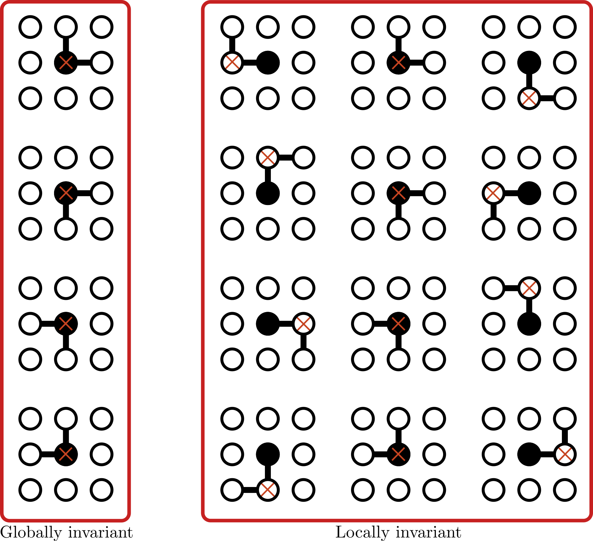
_images/site_centric.png — Illustration of globally-invariant vs locally-invariant clusters. Black sites represent the central sites, while the orange crosses represent the center of the cluster. Any column of in the locally-invariant orbit is a valid choice of globally-invariant clusters.

normalization

The argument is used to specify whether the computed correlation functions should be nomalized by the size of the orbit \(M\) and number of permutations \(P\). If set to True, the normalization consists in multiplying the correlation functions by the factor \(1/(M \cdot \sqrt{P})\). If set to False, the normalization factor is set to \(1\).

per_unitcell

The argument is used to specify whether the computed property should be nomalized by the number of unitcells in the configuration (i.e., the size of the system). If set to True, the computed property results in a density. In the opposite case, if set to False, the property results in an extensive property (i.e., it scales with the size of the system).

embedding_dimensions

It specifies the embedding dimension for each atomic site in the unitcell. The dimensions should be sorted the same way as the atomic sites are sorted in the PRIM file (see build_sitebasis()).

In case two sites are symmetrically equivalent and are assigned two different embedding dimensions, the largest dimension is set to both of them.
In case of an empty list, the embedding dimensions are automatically determined such that the chemical embedding accounts for 95% of the variance.
In case of a list with a single value, this value is used in for each symmetrically unique embedding.
In case of a dimension smaller or equal to 0, the dimension is set to the number of chemical species, i.e., no chemical compression is performed.

The figure below depicts a chemical compression from 4 dimensions to 2 dimensions.

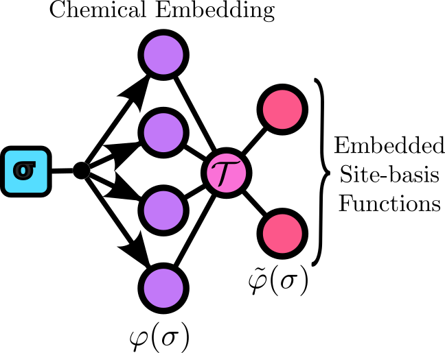
_images/chemical_embedding.png — Illustration of the chemical embedding of a system with 4 chemical species embedded into 2 dimensions, i.e., 2 effective species.

nn_layers

It determines the architecture of the FNN by specifying the number of nodes in each hidden layers. The size of first layer is automatically determined by the number of correlation functions (input features) that are included in the model, which depends on the embedding dimensions and orbits (see build_FNN()). The last layer is always set to 1 as it returns the energy per unitcell. An empty list results in a linear model. The figure bellow depicts such a FNN with 3 hidden layers containing 4 nodes, 4 nodes, and 2 nodes respectively.

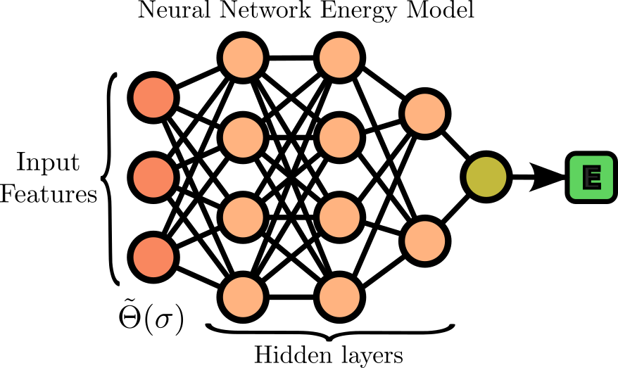
_images/FNN.png — Illustration of a feed-forward neural network with 3 hidden layers

activation

It indicates the PyTorch activation function to be used between all layers within the FNN. The available activation functions can be found in torch.nn.

settings

A path to a yaml file containing all arguments can be given in place of or together with arguments given in the CLI. In case of conflict between arguments given in the settings file and in the CLI, the arguments in the settingsfile have the priority. Missing arguments are set to default values or to the values given in the CLI. Below is an example of such a settings file.

# Prim specifications
prim : "PRIM"                        # Path to the PRIM file
basis: "chebyshev"                   # Full rank basis [`chebyshev`, `occupational`]
orbit_tree_specs:                    # Path to the PRIM file
   orbit_tree_length_filter:         # Constraints on the orbit tree based on the cluster dimensions
       0:                            # Empty cluster
           min_length: 0
           max_length: 0
       1:                            # Point clusters
           min_length: 0
           max_length: 0
       2:                            # Pair clusters
           min_length: 0
           max_length: 10
       3:                            # Triplet clusters
           min_length: 4
           max_length: 8

# ECI neural network specifications
embedding_dimensions: [3]            # Number of embedding dimensions for each site in the unitcell
nn_layers: [32, 32, 8]               # Number of nodes in each hidden layers
activation: "ReLU"                   # Activation function
globally_invariant: false            # Globally-invariant orbits as opposed to locally-invariant (i.e., site-centric) orbits (to be used if using a linear model)

name

It specifies the name of the model once it is built. PyeCE eCE models are saved either as the Pytorch default settings (typically use a .pt or .pth extension) or as a gz-compressed tarfile if the eci model is not built using the from_settings building attribute (use a .tar.gz extension). The tarfile contains 3 files:

prim.json: a json file to be used construct a Prim object.
ece.pth: a PyTorch file to reload the ECI energy model with the correct architecture.
eCE_state.pth: a PyTorch file to reload the weights of the eCE model.

verbose

Set it to print information during the building of the model.

Example: Cr-Mo-Nb-Ta-V-W alloy

In this example, we are interested in the senary BCC Cr-Mo-Nb-Ta-V-W system. We consider pairs and triplet clusters with lengths smaller or equal to 10 Å for the former and 4 Å for the latter, in addition to the empty and point clusters. The 6-dimensional chemical space is embedded into a 3-dimensional subspace, i.e., the embedding dimension is set to 3. Finally, the ECI energy model has 4 hidden layers containing 128 nodes, 128 nodes, 32 nodes, and 8 nodes, respectively, with the ReLU activation function between each layers.

PRIM file

The PRIM file for this system reads:

BCC Cr-Mo-Nb-Ta-V-W
   1.00000000000000
    -1.6535218700000000    1.6535218700000000    1.6535218700000000
     1.6535218700000000   -1.6535218700000000    1.6535218700000000
     1.6535218700000000    1.6535218700000000   -1.6535218700000000
     1
Direct
  0.0000000000000000  0.0000000000000000  0.0000000000000000 Cr Mo Nb Ta V W

CLI command

In order to build the eCE model for this system from the CLI, you can run the following command:

python /pyece/cli/ece.py \
    -p PRIM \
    --basis chebyshev \
    -o '{"orbit_tree_length_filter":{"0": {}, "1": {}, "2": {"max_length": 8}, "3": {"max_length": 4}}}' \
    -e 3 \
    -l 128 128 32 8 \
    -a ReLU \
    -n model_bcc.pth

Settings file

In order to build the eCE model for this system using the yaml settings file, you must create a build_settings.yaml file as follows:

prim : "PRIM"
basis: "chebyshev"
orbit_tree_specs:
   orbit_tree_length_filter:
       0:
           max_length: 0
       1:
           max_length: 0
       2:
           max_length: 10
       3:
           max_length: 4
embedding_dimensions: [3]
nn_layers: [128, 128, 32, 8]
activation: "ReLU"
globally_invariant: false
name: model_bcc.pth

And the model can be built by running the following line

python /pyece/cli/ece.py -s build_settings.yaml