Tutorial
This tutorial constructs an embedded cluster expansion (eCE) model for the BCC Cr-Mo-Nb-Ta-V-W system (A2 structure). The model is trained to predict the formation energy per atom of any configuration of these 6 chemical species on the BCC lattice.
The first thing to do is to activate the pyece conda environement by running the following command:
conda activate pyece
Writing Input Files
In order to construct the eCE model, two files need to be created. As explained in User-guide, these files are the PRIM file and the settings.json file.
PRIM file
The PRIM file describes the primitive crystal structure and the degree of freedom of the sublattices. To construct the file, we use the VASP POSCAR of a relaxed BCC-Nb structure. The underlying lattice corresponds to that of pure Nb. This file now needs to be modified to indicate the degree of freedom, i.e., Cr-Mo-Nb-Ta-V-W, of the lattice (BCC only has one “sublattice”). To do that, the line corresponding to the chemical species (i.e., the 6th line in convensional VASP POSCAR file) needs to be removed. Instead, the permitted chemical species are written after the coordinates of the atomic site. The resulting PRIM file is:
BCC Cr-Mo-Nb-Ta-V-W
   1.00000000000000
    -1.6535218700000000    1.6535218700000000    1.6535218700000000
     1.6535218700000000   -1.6535218700000000    1.6535218700000000
     1.6535218700000000    1.6535218700000000   -1.6535218700000000
     1
Direct
  0.0000000000000000  0.0000000000000000  0.0000000000000000 Cr Mo Nb Ta V W
Note
The chemical species are automatically sorted by alphabetic orther, with the vacancies (labelled as ‘Va’) placed at the end. Sites with no chemical degree of freedom (i.e., only one specie is allowed) are automatically placed at the end of the list of sites.
Settings
The settings are written in a JSON file. The file is divided into two pieces: the “prim” and the “eCE”.
The “prim” part specifies the system of investigation. It gives the path to the PRIM file described above. The Chebyshev basis is used as unprojected site-basis functions. Orbits with a maximum of 3 atoms (body-order of 3) are considered. All pair clusters whose maximum length is smaller or equal to 9 Å and all triplet clusters whose maximum length is smaller or equal to 4 Å are considered in addition to the empty and point clusters.
The “eCE” part specifies the machine-learning model. The embedding dimension is set to 3, i.e., instead of considering the 6 independent chemcial species, the model treates the chemical species as linearly dependent on 3 effective chemcial species. The “effective cluster interactions” (ECI) is evaluated through a feed-forward neural netweork composed of 4 hidden layers composed of 128, 128, 32, and 8 nodes, respectively. Between each layer, the “ReLU” activation is used. Site-centric orbits are constructed.
The resulting JSON file (build_settings.json) is shown below:
# Prim specifications
"path" : "PRIM"                        # Path to the PRIM file
"basis": "chebyshev"                   # Full rank basis [`chebyshev`, `occupational`]
"orbit_tree_specs":
   "orbit_tree_length_filter":         # Constraints on the orbit tree based on the cluster dimensions
      "0":                             # Empty cluster
         "max_length": 0
      "1":                             # Point clusters
         "max_length": 0
      "2":                             # Pair clusters
         "max_length": 9
      "3":                             # Triplet clusters
         "max_length": 4

# ECI neural network specifications
"embedding_dimensions": [3]            # Number of embedding dimensions for each sublattices
"nn_layers": [128, 128, 32, 8]         # Number of nodes in each hidden layers
"activation": "ReLU"                   # Activation function
"globally_invariant": false            # Site centric orbits as opposed to global orbits (to be used if using a linear model)
Constructing the Model
The eCE model is constructed using the built-in from_settings() method. The method takes the settings file written above as input. The following code creates the model:
from pyece.core.clex import eCE

model = eCE.from_settings(path_to_settings = "build_settings.json")
The eCE is composed of four modules:
The
prim: It corresponds to thePrimobject. Printing it yields the following string representation:PRIM ┏━━━━━━━━━━━━━━━━━━━━━━━━━━━━━━━━━━━━━━━━━━━━━━━━━━━━━━━━━━━━━┓ ┃ General: ┃ ┃ -------- ┃ ┃ Space group : Im-3m (229) ┃ ┃ Chemical species : Cr Mo Nb Ta V W ┃ ┃ Chemical indexes 0 1 2 3 4 5 ┃ ┃ Accuracy : 6 digits ┃ ┃ Cutoff : 9 Å ┃ ┃ neighborhood size : 169 atomic sites ┃ ┣━━━━━━━━━━━━━━━━━━━━━━━━━━━━━━━━━━━━━━━━━━━━━━━━━━━━━━━━━━━━━┫ ┃ Lattice: ┃ ┃ -------- ┃ ┃ a -1.65352 1.65352 1.65352 ┃ ┃ b 1.65352 -1.65352 1.65352 ┃ ┃ c 1.65352 1.65352 -1.65352 ┃ ┣━━━━━━━━━━━━━━━━━━━━━━━━━━━━━━━━━━━━━━━━━━━━━━━━━━━━━━━━━━━━━┫ ┃ Basis: ┃ ┃ ------ ┃ ┃ Index Coordinates Equivalency Permitted species ┃ ┃ ------- ------------- ------------- -------------------- ┃ ┃ 0 0 0 0 0 Cr Mo Nb Ta V W ┃ ┗━━━━━━━━━━━━━━━━━━━━━━━━━━━━━━━━━━━━━━━━━━━━━━━━━━━━━━━━━━━━━┛
The first part gives the general information about the lattice, i.e., A2 structure with spacegroup 225. Each chemcial specie is associated to a unique chemcial index. Cr is associated to the index 0, Mo to the index 1, Nb to the index 2, Ta to the index 3, V to the index 4, and W to the index 5. The cutoff radius of interaction is set to 9 Å, which includes 169 neighbor sites. The second part prints the lattice vectors as row-vectors. Finally, the last part prints the sublattices with the degree of freedom associated to each of them. The index correponds to the basis index, while the equivalency correponds to the index of the symmetrically-unique sublattice. In our case, BCC has only one sublattice that can be occupied by Cr, Mo, Nb, Ta, V, or W.
The
sitebasis: It corresponds to theSiteBasisobject. Printing it yields the following string representation:SITE-BASIS ┏━━━━━━━━━━━━━━━━━━━━━━━━━━━━━━━━━━━━━━━━━━━━━━━━━━━━━━━━━━━━━━━━━━━━━━━━━━━━━━━━━━┓ ┃ Embedding Dimensions: ┃ ┃ --------------------- ┃ ┃ Symmetry equivalency 0 : 0 1 2 3 4 5 -> 3 embedding dimensions ┃ ┣━━━━━━━━━━━━━━━━━━━━━━━━━━━━━━━━━━━━━━━━━━━━━━━━━━━━━━━━━━━━━━━━━━━━━━━━━━━━━━━━━━┫ ┃ Site-basis Functions: ┃ ┃ --------------------- ┃ ┃ Chemical indexes : 0 1 2 3 4 5 ┃ ┃ ┃ ┃ 1.0000 1.0000 1.0000 1.0000 1.0000 1.0000 ┃ ┃ ┃ ┃ Sites of equivalency 0 : 0.8399 -0.3814 0.5427 -0.2961 1.1506 -1.8556 ┃ ┃ 1.1037 0.6773 -0.9937 -1.7018 0.3538 0.5607 ┃ ┗━━━━━━━━━━━━━━━━━━━━━━━━━━━━━━━━━━━━━━━━━━━━━━━━━━━━━━━━━━━━━━━━━━━━━━━━━━━━━━━━━━┛
The first part is a reminder of the system. The symmetrically unique sublattices (equivalency) are indicated together with the indexes of the species allowed on these sites. As mentioned above, the BCC structure has only one sublattice. The second part prints the site-basis functions. Each row corresponds to one site-basis function, while each column corresponds to the representation of one chemical species. Each symmetrically unique sublattice is described by its own set of site-basis function. The constant site-basis function (i.e., the first row) is common to all sublattices. It formally allows for the notion of cluster (the sites not included in the cluster are assigned to the constant site-basis function, see Description). The site-basis functions are initialized acccording to the chemical species to already include chemcial information (see the
chemical_preconditioning()). Hence, the number of embedding dimensions is 3, i.e., two site-basis functions in addition to the constant site-basis function.The
features: It corresponds to theFeaturesobject. Printing it yields the following string representation:FEATURES ┏━━━━━━━━━━━━━━━━━━━━━━━━━━━━━━━━━━━━━━━━━━━━━━┓ ┃ Orbit Orbit Number of Cluster ┃ ┃ index size feautures composition ┃ ┃ ------- ------- ----------- ------------- ┃ ┃ 0 1 1 ┃ ┃ 1 1 2 0 ┃ ┃ 2 8 3 0 - 0 ┃ ┃ 3 6 3 0 - 0 ┃ ┃ 4 12 3 0 - 0 ┃ ┃ 5 24 3 0 - 0 ┃ ┃ 6 8 3 0 - 0 ┃ ┃ 7 6 3 0 - 0 ┃ ┃ 8 24 3 0 - 0 ┃ ┃ 9 24 3 0 - 0 ┃ ┃ 10 24 3 0 - 0 ┃ ┃ 11 24 3 0 - 0 ┃ ┃ 12 8 3 0 - 0 ┃ ┃ 13 36 6 0 - 0 - 0 ┃ ┗━━━━━━━━━━━━━━━━━━━━━━━━━━━━━━━━━━━━━━━━━━━━━━┛
This string representation summarizes the correlation functions considered in the model. As stated in settings.json, the descriptors correspond to the empty cluster (1 correlation function/feature), the point cluster (2 correlation functions/features), 11 pair clusters (all with 3 associated correlation functions/features), and one triplet cluster (6 correlation functions/features). All these clusters are composed of sites belonging to the same symmetrically unique sublattice sublattice (again, there is only one in BCC).
The
eci: It corresponds to the effective cluster ineteractions neural netweok object. Its Pytorch string representation yields:Sequential( (0): Linear(in_features=42, out_features=128, bias=False) (1): ReLU() (2): Linear(in_features=128, out_features=128, bias=True) (3): ReLU() (4): Linear(in_features=128, out_features=32, bias=True) (5): ReLU() (6): Linear(in_features=32, out_features=8, bias=True) (7): ReLU() (8): Linear(in_features=8, out_features=1, bias=True) )
The neural network is composed of 5 matrices with 42x128, 128x128, 128x32, 32x8, and 8x1 shapes, separated by ReLU actication functions. The number of input features of the first matrix corresponds to the number of correlation functions (i.e., features) computed by the
Featuresobject. The predicted property being a scalar (i.e., the formation energy per atom), the number of output features of the last matrix is 1.
Tip
The command line interface can also be used directly for this task, using the build command as (see Construction of an eCE model):
python /pyece/cli/ece.py build -s build_settings.yaml
Constructing the Database
In order to train the model, a database of several configurations whose formation energy per atom is known needs to be constructed. Typically, ab initio methods such as DFT are employed for this task. The output structures of these methods need to be transformed into input features for the eCE model. The mapping module is used to map the possibly relaxed structures onto an ideal structure compatible with the lattice defined in the prim object. Input features for the eCE model are then converted from the ideal structure by the configurations module.
Note
The output structures resulting from ab initio methods are generally relaxed structures. During relaxation, lattice deformations and atomic displacements are often applied to the ideal structure.
Mapping Structures
The following structure corresponds to the output of a relaxation calculation using DFT:
Cr Ta V W
1.0
   3.0919046500000000    0.0000000000000000    0.0000000000000000
   0.0000000000000000    3.0653813699999999   -3.0653813699999999
  -1.5459523200000000    1.6048491000000000    4.6702304699999999
Cr Ta V W
 1  1 1 1
direct
   0.2504773800000000    0.7504773800000000    0.5009547600000001 Cr
   0.7501208200000000    0.2501208200000000    0.5002416500000000 Ta
   0.5095649500000000    0.5095649500000000    0.0191299000000000 V
   0.9898368400000001    0.9898368400000001    0.9796736900000000 W
The formation energy per atom yields -0.03085 eV/at. Reading the output structure with Pymatgen structure, the Config object is constructed using the built-in from_structure() method. The following code maps the structure and creates the Config object:
from pymatgen.core import Structure
from pyece.core.configurations import Config

poscar = """Cr Ta V W
            1.0
            3.0919046500000000    0.0000000000000000    0.0000000000000000
            0.0000000000000000    3.0653813699999999   -3.0653813699999999
           -1.5459523200000000    1.6048491000000000    4.6702304699999999
            Cr Ta V W
            1  1 1 1
            direct
            0.2504773800000000    0.7504773800000000    0.5009547600000001 Cr
            0.7501208200000000    0.2501208200000000    0.5002416500000000 Ta
            0.5095649500000000    0.5095649500000000    0.0191299000000000 V
            0.9898368400000001    0.9898368400000001    0.9796736900000000 W"""
structure = Structure.from_str(poscar, fmt="poscar")
config = Config.from_structure(structure, eCE.prim)
The config object corresponds to an ordering on the supercell whose transformation matrix \(T\) is:
The object yields the following string representation:
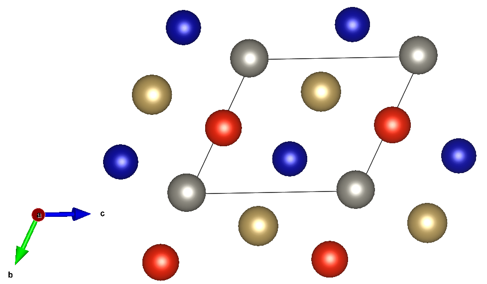
                           CONFIGURATION TaVCrW
┏━━━━━━━━━━━━━━━━━━━━━━━━━━━━━━━━━━━━━━━━━━━━━━━━━━━━━━━━━━━━━━━━━━━━━━━━━┓
┃ General:                                                                ┃
┃ --------                                                                ┃
┃ Composition          :   Cr  Mo  Nb  Ta  V  W                           ┃
┃                           1   0   0   1  1  1                           ┃
┃ Number of unitcells  :   4 neighborhoods                                ┃
┃ Neighborhood size    :   169 atoms                                      ┃
┣━━━━━━━━━━━━━━━━━━━━━━━━━━━━━━━━━━━━━━━━━━━━━━━━━━━━━━━━━━━━━━━━━━━━━━━━━┫
┃ Lattice:                                                                ┃
┃ --------                                                                ┃
┃ a           3.30704  0         0                                        ┃
┃ b            0        3.30704  -3.30704                                 ┃
┃ c           -1.65352  1.65352   4.96057                                 ┃
┣━━━━━━━━━━━━━━━━━━━━━━━━━━━━━━━━━━━━━━━━━━━━━━━━━━━━━━━━━━━━━━━━━━━━━━━━━┫
┃ Basis:                                                                  ┃
┃ ------                                                                  ┃
┃ Index    Coordinates       Unitcell    Basis index    Chemical species  ┃
┃ -------  ---------------  ----------  -------------  ------------------ ┃
┃ 0        0.25  0.75  0.5      0             0                Cr         ┃
┃ 1        0.75  0.25  0.5      1             0                Ta         ┃
┃ 2        0.5   0.5   0        2             0                V          ┃
┃ 3        0     0     0        3             0                W          ┃
┗━━━━━━━━━━━━━━━━━━━━━━━━━━━━━━━━━━━━━━━━━━━━━━━━━━━━━━━━━━━━━━━━━━━━━━━━━┛
As described by the transformation matrix \(T\), the structure corresponds to a supercell of size 4 (i.e., 4 times the primitive structure). From Config objects, the input features to the eCE model are simply computed as:
input_features = config.get_neighborhood_occupations()
And the predicted formation energy of the configuration can be computed as:
formation_energy = eCE(input_features).mean()
Note
The model computes an effective formation energy per atom for each unitcell and then sums them to estimate the global formation energy of the configuration (or take the mean of them in order to get the formation energy per unitcell). If the formation energy per atom of several configurations are simultaneously computed, we need to inform the model which unitcells belong to the same configuratrion. This can conveniently be achieved by the ClexInput object using the from_list_configs() method.
Building Databases
The training stage requires several configurations and an associated property (e.g., the formation energy per atom) that constitutes the database. The ConfigData object basically links the Config to a property and (optionally) a weight, here the formation energy per atom:
from pyece.learn.data import ConfigData

formation_energy_per_atom = -0.03085
data = ConfigData(config, formation_energy_per_atom)
dct = data.as_dict()
In the last line, the ConfigData is stored as a MSONable dictionary.
Tip
The command line interface can also be used directly for this task, using the data command. When a batch of configuration needs to be mapped onto the prim structure, a file containing the paths to the files with the structures, the properties, and (optionally) the weights on each line can be used to create a database at once.
Here is an example of the creation of a database in the senary BCC system. Pure elements are given a weight of 5.0 while the others are assigned the default weight of 1.0:
/pyece/example/bcc/POSCAR/Cr.vasp       -9.51213908     5.0
/pyece/example/bcc/POSCAR/Mo.vasp       -10.93448903    5.0
/pyece/example/bcc/POSCAR/Nb.vasp       -10.21577832    5.0
/pyece/example/bcc/POSCAR/Ta.vasp       -11.81286982    5.0
/pyece/example/bcc/POSCAR/V.vasp        -8.99029792     5.0
/pyece/example/bcc/POSCAR/W.vasp        -12.95502032    5.0
/pyece/example/bcc/POSCAR/CrNb.vasp     -19.41790023
/pyece/example/bcc/POSCAR/CrV.vasp      -18.66543936
/pyece/example/bcc/POSCAR/CrW.vasp      -22.23796813
/pyece/example/bcc/POSCAR/MoNb.vasp     -21.30885536
/pyece/example/bcc/POSCAR/MoTa.vasp     -23.12021311
/pyece/example/bcc/POSCAR/MoW.vasp      -23.90862633
/pyece/example/bcc/POSCAR/NbTa.vasp     -22.02874408
/pyece/example/bcc/POSCAR/TaV.vasp      -20.75874751
/pyece/example/bcc/POSCAR/TaW.vasp      -24.88562793
/pyece/example/bcc/POSCAR/VW.vasp       -22.07277700
the database database.json is then built by running the command (see Train an eCE model):
python /pyece/cli/ece.py data -b data_batch.txt -a -n database.json
The -a argument is used to automatically determine the end configurations to compute the formation energy. It yields:
Automated references:
 - Cr: -9.51213908
 - Mo: -10.93448903
 - Nb: -10.21577832
 - Ta: -11.81286982
 - V: -8.99029792
 - W: -12.95502032
Loading Training Datasets
In order to train the model, a training dataset composed of many ConfigData objects needs to be build. A list of ConfigData dictionaries with ~4000 different configurations is available in the example/bcc folder. PyeCE uses the Pytorch library to train the model. Pytorch Dataloaders are build from the pyece ConfigDataset object as:
import json
from pyece.learn.data import ClexData, ClexDataset
from torch import utils

# Read the training dataset from ClexData
with open("example/bcc/train_dataset.json", "r") as f:
    list_dct = json.load(f)
    f.close()
list_configdata_train = []
for dct in list_dct:
    list_configdata_train.append(ConfigData.from_dict(dct))

# Read the validation dataset from ClexData
with open("example/bcc/valid_dataset.json", "r") as f:
    list_dct = json.load(f)
    f.close()
list_configdata_valid = []
for dct in list_dct:
    list_configdata_valid.append(ConfigData.from_dict(dct))

# Read the test dataset from ClexData
with open("example/bcc/test_dataset.json", "r") as f:
    list_dct = json.load(f)
    f.close()
list_configdata_test = []
for dct in list_dct:
    list_configdata_test.append(ConfigData.from_dict(dct))

# Build ClexDataset objects
dataset_train = ClexDataset.build_dataset(list_configdata_train)
dataset_val = ClexDataset.build_dataset(list_configdata_valid)
dataset_test = ClexDataset.build_dataset(list_configdata_test)

# Build Pytorch Dataloader objects
dataloader_train = utils.data.DataLoader(dataset_train, batch_size=50, shuffle=True)
dataloader_test = utils.data.DataLoader(dataset_test, batch_size=50, shuffle=False)
dataloader_valid = utils.data.DataLoader(dataset_val, batch_size=50, shuffle=False)
The Pytorch Dataloader objects automatically construct batches of 50 configurations. These batches return the input features related to the configurations and the labels (i.e., the formation energies per atom).
Training the Model
Training the model consists in determining the optimal embedding site-basis functions and the effective cluster interactions neural network. Here, the ladder training method is used. Ladder training consists in training a first model with a restricted set of correlation functions corresponding to simple compact clusters. Strating from this parameterization, the number of correaltion functions is increased a little to include less simple and compact clusters and the model is trained again. This iterative process is performed until training a model that contains all correlation functions in Features.
The Pytorch Optimizer chosen for this task is the Adam algorithm with L2-regularization of \(10^{-6}\). Schedulers are also used to adjust the learning rate as a the number of steps increases. Here, a simple Multi-step scheduler is used. Finally, the Pytorch Loss Function chosen for the training is the MSE. For each ladder step, both the optimizer and the scheduler need to be given. The first ladder step optimization uses 100 steps with a learning rate going from \(10^{-2}\) to \(10^{-4}\). During the other ladder step optimizations, the learning rate only varies from \(10^{-3}\) to \(10^{-4}\). The ladder steps are chosen to contain the 3, 5, 7, 9, 11, 13, and finally 14 first orbits as arranged in Features.
The training is performed by running the following lines:
from torch import nn, optim
from pyece.learn.train import test, ladder_optimize

# Define ladder steps
ladder_step_orbit_assignment = [3, 5, 7, 9, 11, 13, 14]

# Define the optimizers and schedulers for each ladder step
optimizer1 = optim.Adam(eCE.parameters(), lr=0.01, amsgrad=True, weight_decay=1e-6)
scheduler1 = optim.lr_scheduler.MultiStepLR(optimizer1, milestones=[60, 90], gamma=0.1)
list_optimizers = [optimizer1]
list_schedulers = [scheduler1]
for ladder_step in range(len(ladder_step_orbit_assignment) - 1):
    optimizer2 = optim.Adam(eCE.parameters(), lr=0.001, amsgrad=True, weight_decay=1e-6)
    list_optimizers.append(optimizer2)
    list_schedulers.append(
        optim.lr_scheduler.MultiStepLR(optimizer2, milestones=[30], gamma=0.1)
    )
list_early_stopping = [
    EarlyStopping(patience=10, verbose=True) for _ in range(len(list_optimizers))
]

# Define number optimization epochs
list_n_epochs=[100] + [40] * (len(ladder_step_orbit_assignment) - 1)

# Ladder optimization
losses = ladder_optimize(
    dataloader_train,
    eCE,
    nn.MSELoss(),
    list_optimizers,
    list_schedulers,
    list_n_epochs=list_n_epochs,
    ladder_step_orbit_assignment=ladder_step_orbit_assignment,
    test_dataloader=dataloader_test,
    valid_dataloader=dataloader_valid,
    list_early_stopping=list_early_stopping,
    device=device,
)

# Print RMSE
print(
    "\nFinal training error (RMSE): %.2f meV\n"
    % (np.sqrt(test(dataloader_train, eCE, nn.MSELoss(), device)) * 1000),
)
print(
    "\nFinal validation error (RMSE): %.2f meV\n"
    % (np.sqrt(test(dataloader_valid, eCE, nn.MSELoss(), device)) * 1000),
)
print(
    "\nFinal test error (RMSE): %.2f meV\n"
    % (np.sqrt(test(dataloader_test, eCE, nn.MSELoss(), device)) * 1000),
)

# Save trained eCE model
eCE.tar_save("fitted_model.tar.gz")
The last line stores the model as tar.gz. When the verbosity is on, the training process can be followed as:
Entering ladder training step 0
-------------------------------
Included orbits:
   - Orbit_0_0
   - Orbit_1_0
   - Orbit_2_0

Epoch 0
Learning rate   1.00e-02
Validation loss decreased (inf --> 0.02267715).  Saving model ...
Train Error: 0.02717056
Valid Error: 0.02267715

Epoch 1
Learning rate   1.00e-02
Validation loss decreased (0.02267715 --> 0.00178792).  Saving model ...
Train Error: 0.00098149
Valid Error: 0.00178792

Epoch 2
Learning rate   1.00e-02
Validation loss decreased (0.00178792 --> 0.00049585).  Saving model ...
Train Error: 0.00044463
Valid Error: 0.00049585

Epoch 3
Learning rate   1.00e-02
Validation loss decreased (0.00049585 --> 0.00042622).  Saving model ...
Train Error: 0.00027773
Valid Error: 0.00042622

Epoch 4
Learning rate   1.00e-02
Validation loss decreased (0.00042622 --> 0.00029981).  Saving model ...
Train Error: 0.00026116
Valid Error: 0.00029981

...

Epoch 38
Learning rate   1.00e-04
EarlyStopping counter: 1 out of 10
Train Error: 0.00000312
Valid Error: 0.00000817

Epoch 39
Learning rate   1.00e-04
EarlyStopping counter: 2 out of 10
Train Error: 0.00000303
Valid Error: 0.00000788

Epoch 40
Learning rate   1.00e-04
Validation loss decreased (0.00000787 --> 0.00000786).  Saving model ...
Train Error: 0.00000297
Valid Error: 0.00000786

Final training error (RMSE): 1.72 meV


Final validation error (RMSE): 2.80 meV


Final test error (RMSE): 2.43 meV
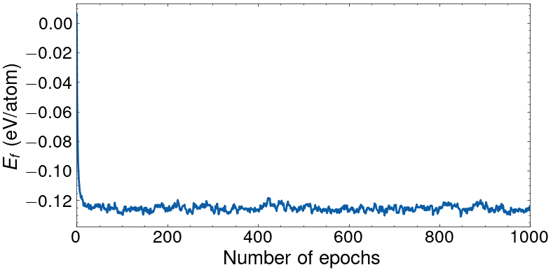
The result of the optimization is illustrated below. The training error is 1.72meV, the validation error is 2.80meV, and the test error is 2.43meV. The early-stopping ensures that the validation loss does not increase, but the training error can still increase.

Tip
The command line interface can also be used directly for this task, using the fit command as (see Train an eCE model):
python /pyece/cli/ece.py fit -s fit_settings.yaml
where the settings read as follows:
# Datasets
train_file: train_dataset.json
valid_file: valid_dataset.json
test_files:
- test_dataset.json

# Fitting parameters
batch_size: 50
ladder_steps: [3, 5, 7, 9, 11, 13, 14]
epochs: [100, 40, 40, 40, 40, 40, 40]
lr: [0.01, 0.001, 0.001, 0.001, 0.001, 0.001, 0.001]
weight_decay: 1e-6
optimizers:
   Adam:
      amsgrad: true
schedulers:
- MultiStepLR:
   milestones: [60, 90]
   gamma: 0.1
- MultiStepLR:
   milestones: [30]
   gamma: 0.1
- MultiStepLR:
   milestones: [30]
   gamma: 0.1
- MultiStepLR:
   milestones: [30]
   gamma: 0.1
- MultiStepLR:
   milestones: [30]
   gamma: 0.1
earlystopping_patience: 10

# Name of the fitted model
name: fitted_model.tar.gz
Monte Carlo Simulations
The model is now ready to be used. Here, a Monte Carlo simulation in the semi-grand canonical ensemble is illustrated. In this ensemble, the temperature, the total number of atoms, as well as all degrees of freedom of chemical potentials except one are fixed, while the internal energy, the composition, and the left chemical potential can vary. It is usually more convenient to work with the chemical potential differences. Let’s investigate the alloy at 1000K with the chemical potential differences fixed to 0. The initial configuration contains 2000 atoms with random occupation at a composition close to equiatomic. The following code shows the construction of the random configuration and carries out 1000 Monte Carlo epochs using the SemiGrandCanonical operator:
from pyece.core import clex
from pyece.core.configurations import Config
from pyece.montecarlo.mcmc import SemiGrandCanonical
import numpy as np

# Load model
eCE = clex.eCE.tar_load("fitted_model.tar.gz")
print(eCE.prim)

# Construct random configuration
transformation = np.array([[0, 1, 1], [1, 0, 1], [1, 1, 0]]) * 10
labels = np.random.choice(
    eCE.prim.elements, size=np.rint(np.linalg.det(transformation)).astype(int)
)
structure = eCE.prim.structure.make_supercell(
    transformation, to_unit_cell=True, in_place=False
)
for site_index, specie in enumerate(labels):
    structure.replace(site_index, species=specie)
config = Config.from_structure(structure, eCE.prim)

# Construct MC object
mc = SemiGrandCanonical(
    model=eCE,
    config=config,
    temperature=1000,
    mu_tilde=np.array([0, 0, 0, 0, 0]),
    chemical_transformation=np.eye(6)[:5],
    device="cuda",
)

# Carry out the MC simulation
mc(N_samples=1000, sampling_frequency=mc.N_sites)
Here, the chemical_transformation is the linear combination that transforms the chemical potentials into the difference of chemical potentials, with the chemical potential associated to the last specie (i.e., W) being the backgroud. One Monte carlo epoch corresponds to 2000 Monte Carlo swap trials (such that a swap at every site is proposed in average). The initial state is a random alloy with nearly equiatomic composition (\(\text{Cr}_{0.18}\) \(\text{Mo}_{0.16}\) \(\text{Nb}_{0.16}\) \(\text{Ta}_{0.17}\) \(\text{V}_{0.18}\) \(\text{W}_{0.15}\)) with a predicted formation energy of 6.2 meV/at. The final state had the composition \(\text{Cr}_{0.00}\) \(\text{Mo}_{0.41}\) \(\text{Nb}_{0.10}\) \(\text{Ta}_{0.30}\) \(\text{V}_{0.03}\) \(\text{W}_{0.16}\) with a predicted formation energy of -123.8 meV/at. Printing the SemiGrandCanonical object yields:
                MONTE CARLO ENSEMBLE
┏━━━━━━━━━━━━━━━━━━━━━━━━━━━━━━━━━━━━━━━━━━━━━━━━━━━━━━━━━━━┓
┃ General:                                                  ┃
┃ --------                                                  ┃
┃ Temperature (beta)           :   1000.000 K (11.605 eV/K) ┃
┃ Total number of sites        :   2000                     ┃
┃ Number of variable sites     :   2000                     ┃
┃ Number of samples generated  :   1000                     ┃
┣━━━━━━━━━━━━━━━━━━━━━━━━━━━━━━━━━━━━━━━━━━━━━━━━━━━━━━━━━━━┫
┃ Fixed Variables:                                          ┃
┃ ----------------                                          ┃
┃ temperature         :   1000                              ┃
┃ beta                :   11.604518121745585                ┃
┃ mu_tilde            :   [0.0, 0.0, 0.0, 0.0, 0.0]         ┃
┃ N_sites             :   2000                              ┃
┣━━━━━━━━━━━━━━━━━━━━━━━━━━━━━━━━━━━━━━━━━━━━━━━━━━━━━━━━━━━┫
┃ Fluctuating Variables:                                    ┃
┃ ----------------------                                    ┃
┃ E                         :   -0.1252    ±   0.003862     ┃
┃ N_Cr                      :    0.001498  ±   0.002507     ┃
┃ N_Mo                      :    0.4098    ±   0.009449     ┃
┃ N_Nb                      :    0.09723   ±   0.006597     ┃
┃ N_Ta                      :    0.3052    ±   0.009842     ┃
┃ N_V                       :    0.0393    ±   0.006769     ┃
┃ N_W                       :    0.1469    ±   0.009173     ┃
┣━━━━━━━━━━━━━━━━━━━━━━━━━━━━━━━━━━━━━━━━━━━━━━━━━━━━━━━━━━━┫
┃ Current State:                                            ┃
┃ --------------                                            ┃
┃ Composition       :   Cr   Mo   Nb   Ta   V    W          ┃
┃                        4  815  193  603  71  314          ┃
┃ Energy            :   -0.123811 eV/unitcell               ┃
┗━━━━━━━━━━━━━━━━━━━━━━━━━━━━━━━━━━━━━━━━━━━━━━━━━━━━━━━━━━━┛
The evolution of the formation energy with the number of epochs carried out is shown in the figure below.
Cool-down runs
We are often interested in performing successive MCMC simulation with one state variable being scanned from two different values. This is typically the case when performing simulated annealing. Here is an example of a cool-down run from high to low temperature in the Canonical ensemble at equiatomic concentration. The cooling() function is meant for this task.
The following lines can be used to perform such a simulated annealing with the temperature ranging from 20’000 to 500K (logarithic spacing from 20’000 to 5’000K and linear spacing from 5’000 to 500K). The short range order parameters for the nearest neighbors (i.e., for pair clusters smaller than 3.0 Å) are also computed:
import numpy as np
from pyece.core import clex
from pyece.montecarlo.mcmc import Canonical
from pyece.montecarlo.run import cooling
from pyece.montecarlo.properties import SRO
from pyece.core.configurations import Config

# Load model
eCE = clex.eCE.tar_load("fitted_model.tar.gz")

# Construct equiatomic configuration
transformation = np.array([[0, 1, 1], [1, 0, 1], [1, 1, 0]]) * 10
structure = eCE.prim.structure.make_supercell(
    transformation, to_unit_cell=True, in_place=False
)
indexes = np.linspace(0, 2000, 7).astype(int)
for id1, id2, elem in zip(indexes[:-1], indexes[1:], eCE.prim.elements):
    for site in range(id1, id2):
        structure.replace(site, elem)
config = Config.from_structure(structure, eCE.prim)

# Construct MC object
mc = Canonical(
    model=eCE,
    config=config,
    temperature=20000,
    device="cuda",
)

# Construct the SRO calculator
sro = SRO(3.0)
sro.set_calculator(eCE.prim, config.get_structure())

# Temperature scan
T = (
    np.logspace(np.log10(20000), np.log10(5000), 10)[:-1].tolist()
    + np.linspace(5000, 500, 46).tolist()
)

# Carry out the MC simulation
data = cooling(
    mc=mc,
    temperatures=T,
    precision={"<E>": 1e-3},
    list_properties=[sro],
    N_uncorrelated_samples=50,
    min_samples=50,
    max_samples=2000,
    path_to_result_data="results.json",
    path_to_last_config="config.json",
)
The cooling simulation can be followed as:
MC simulation at temperature: 20000.0
42 uncorrelated samples out of 50 samples with equilibration time 1 (Time per MC step: 2.053e-04) ===> Status: incomplete
 - <E> : 5.252809e-04
46 uncorrelated samples out of 59 samples with equilibration time 1 (Time per MC step: 1.549e-04) ===> Status: incomplete
 - <E> : 4.854692e-04
51 uncorrelated samples out of 64 samples with equilibration time 1 (Time per MC step: 1.553e-04) ===> Status: complete
 - <E> : 4.513824e-04

MC simulation at temperature: 17144.9
50 uncorrelated samples out of 50 samples with equilibration time 1 (Time per MC step: 1.546e-04) ===> Status: complete
 - <E> : 5.079513e-04

MC simulation at temperature: 14697.3
45 uncorrelated samples out of 50 samples with equilibration time 1 (Time per MC step: 1.543e-04) ===> Status: incomplete
 - <E> : 4.878074e-04
48 uncorrelated samples out of 49 samples with equilibration time 7 (Time per MC step: 1.559e-04) ===> Status: incomplete
 - <E> : 5.087038e-04
54 uncorrelated samples out of 57 samples with equilibration time 1 (Time per MC step: 1.571e-04) ===> Status: complete
 - <E> : 4.485589e-04

MC simulation at temperature: 12599.2
50 uncorrelated samples out of 50 samples with equilibration time 1 (Time per MC step: 1.545e-04) ===> Status: complete
 - <E> : 4.014714e-04

...

MC simulation at temperature: 600.0
19 uncorrelated samples out of 19 samples with equilibration time 32 (Time per MC step: 1.546e-04) ===> Status: incomplete
 - <E> : 5.015206e-04
19 uncorrelated samples out of 46 samples with equilibration time 34 (Time per MC step: 1.515e-04) ===> Status: incomplete
 - <E> : 6.004352e-04
20 uncorrelated samples out of 141 samples with equilibration time 12 (Time per MC step: 1.543e-04) ===> Status: incomplete
 - <E> : 8.127958e-04
66 uncorrelated samples out of 350 samples with equilibration time 13 (Time per MC step: 1.538e-04) ===> Status: complete
 - <E> : 3.909492e-04

MC simulation at temperature: 500.0
8 uncorrelated samples out of 8 samples with equilibration time 43 (Time per MC step: 1.507e-04) ===> Status: incomplete
 - <E> : 7.657233e-04
12 uncorrelated samples out of 71 samples with equilibration time 16 (Time per MC step: 1.546e-04) ===> Status: incomplete
 - <E> : 8.827466e-04
26 uncorrelated samples out of 307 samples with equilibration time 1 (Time per MC step: 1.512e-04) ===> Status: incomplete
 - <E> : 7.316812e-04
58 uncorrelated samples out of 413 samples with equilibration time 177 (Time per MC step: 1.564e-04) ===> Status: complete
 - <E> : 4.018644e-04
For each temperature, the simulation stop either when 50 uncorrelated samples are produced and the size of the confidence interval on the average formation energy <E> has reached the desired precision of 0.001 eV, or when the maximum number of samples (set to 2’000) is reached. It can be seen that at high temperatures the samples are barely correlated, while at low temperatures the auto-correlation time is close to 10 samples. Processed data are saved in the results.json file. All fluctuating variables (i.e., properties corresponding to ensemble averages) are returned in the form of a dictionary containing the mean value and the confidence interval. In addition, an estimator of the variance is computed as well for the fluctuating variables (e.g., in the case of the Canonical ensemble, the fluctuating variable is the energy and both an estimator for the average energy <E> and an estimator for the variance <E E>-<E><E> are computed).
The result of the simulation is shown in the figure below.
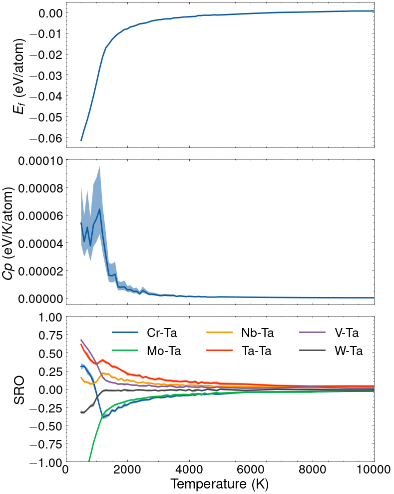
Result of a simulated annealing in the canonical ensemble for the equiatomic CrMoNbTaVW alloy.
Tip
The command line interface can also be used directly for this task, using the mcmc command as (see Finite-temperature simulations):
python /pyece/cli/ece.py fit -s mcmc_settings.yaml
where the settings read as follows:
# Model
model: "fitted_model.tar.gz"
device: "cuda"

# Thermodynamics
ensemble: "Canonical"
increment:
 - mode: "logarithmic"
   number: 10
   initial:
      temperature: 20000
   final:
      temperature: 5000
 - mode: "linear"
   number: 46
   initial:
      temperature: 5000
   final:
      temperature: 500
composition: [1, 1, 1, 1, 1, 1]
supercell: [[0, 10, 10], [10, 0, 10], [10, 10, 0]]
properties:
   SRO:
      cutoff: 3.0

# Simulation
precision:
   <E>: 1e-3
n_uncorrelated: 50
min: 50
max: 2000

# Global
path: results.json
verbose: True
The command can be used for other scans as well, e.g., scanning along a composition path in the Canonical ensemble or along a modified chemical potential in the semi-grand Canonical ensemble.